Where is it worth training the model?
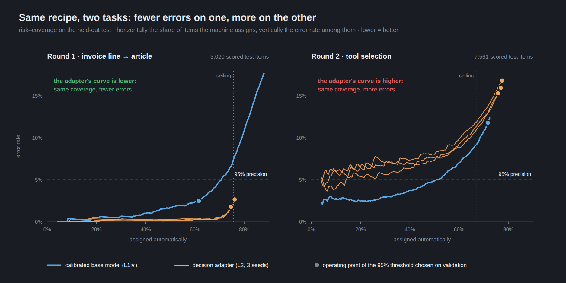
The same decision adapter on two tasks: on one it automates 13.7 points more, on the other it does worse than the untrained model.
On 5 October, at the end of our article on decision models, we promised to try our own idea: a decision adapter on the model we already serve. We also promised to report back if it didn’t work. Both promises are now kept. The same small adapter clearly won on one task and did worse than the untrained model on the other.
Put together, the two results taught us what we think matters most: where it is worth training at all. This is the short version; the long one, with methodology and limitations, is in our research report (in Hungarian) at docai.hu/kutatas.
What we tried
We run a Qwen3.6-35B-A3B under vLLM on our DGX Spark every day. On top of it we trained a small LoRA adapter that, instead of chatting, returns a single decision: the letter of one of the 2–10 offered options, or none of these. Each answer comes with a probability, so we can put a threshold on it: if the model is not confident enough, the decision goes to a person.
The yardstick was the same on both tasks: how many cases the system handles automatically if 95% of those decisions must be correct. The baseline was not the raw model, but the same model without any training, carefully calibrated. That means asking about the options in four different orders, averaging the answers, and adjusting the probabilities on a separate data set. It is cheap, and it is the best we can get out of the model without training.
In both rounds we fixed the success criteria before measuring, including what would happen if the adapter failed.
Invoice line → catalogue article: it won
The first task is matching the line items of purchase invoices to the article catalogue. For each invoice line the system proposes candidate articles; the model has to pick the right one, or say that none of them is it. The measurement ran on synthetic data generated from the aggregated purchasing profile of a real business.
| calibrated base model | decision adapter | |
|---|---|---|
| lines assigned automatically at the 95% target | 61.6% | 75.2% |
| the same with 16 unseen suppliers | 56.8% | 76.3% |
| “none of these” cases recognised | 43% | 96% |
| error rate at 70% coverage | 4.8% | 0.4–0.5% |
The gain is 13.7 percentage points, and 19.5 points with unseen suppliers. Almost all of it comes from the adapter recognising when the right article is not on the list, where the untrained model simply picked one of the offered articles. The adapter and the data set are public on Hugging Face.
Tool selection: it got worse
The second task: given a request, which tool should the agent call, if any? The same recipe, on public data (BFCL, When2Call, xLAM, the Hungarian part of MASSIVE) plus Hungarian requests for our own 62-tool catalogue. The test set had 10,013 items.
| calibrated base model | decision adapter | |
|---|---|---|
| requests assigned automatically | 71.7% | 76.7% |
| of which correct (target: 95%) | 88.2% | 84.0% |
| error rate at 50% coverage | 4.9% | 7.3–8.0% |
| “no suitable tool” recognised | 76.2% | 67.3% |
The adapter assigned more requests, but less accurately, and it recognised the “no suitable tool” cases less often. At equal coverage its error rate was higher too. By the rule fixed before the measurement, it failed.
The table hides a second uncomfortable fact: even the untrained model missed the 95% target. We had chosen the threshold on a data set whose “no suitable tool” cases looked different from the test’s.
Both tasks in one chart: the lower the curve, the fewer the errors at the same share of automated decisions.
Why did the result flip?
First: in tool selection there was little left to gain. Whenever a suitable tool existed, the untrained model already assigned 93–100% of requests with 97–100% precision. The base model has clearly been trained a lot on tool calling, and not at all on matching invoice lines to articles. On the first task it had room to improve; on the second it was already close to the ceiling.
Second: the training showed the wrong kind of “none of these”. 80% of the training cases without a suitable tool were artificial: the same request, with the right tool removed from the list. What the model learned from this is: if a similar tool is there, call it. The test, however, contained genuinely irrelevant requests next to tools that looked close but did not fit. In the first task, the test’s “none of these” cases were built exactly like the training ones, so there this did no harm.
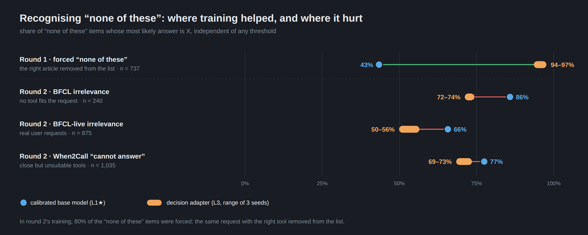
A third effect also showed up: on the Hungarian requests the adapter had learned some wrong labels of the source data set. Where we had corrected a label, it confidently gave the old one.
A model distilled with soft targets is no better
An obvious objection is that the training method was the problem: a model that learns a teacher’s full probability distribution might keep its calibration. There is a public test for that. JEV-27B is an open, distilled version of the closed Jev model (released by AutoTrust AI, not by TypeSafe), and its authors published the model’s answer probabilities on a large benchmark. We compared the models on the same When2Call items.
| separation (AUROC) | false calls at 95% correct calls | |
|---|---|---|
| calibrated base model | 0.964 | 14.1% |
| our decision adapter | 0.945–0.959 | 15.7–17.3% |
| JEV-27B | 0.949 | 37.3% |
JEV-27B lands at the level of our adapter, and both fall short of the untrained, calibrated model. That is not JEV’s fault: its model card measures something else, namely faithfulness to the teacher and accuracy on a fixed set of options. But it does show that soft targets alone do not protect against the “no suitable tool” trap.
What we decided
For matching invoice lines to articles, the decision adapter is a real gain and it stays. The tool-selection adapter will not be published: on the test, the calibrated base model is better, and anyone downloading the adapter would be worse off with it. In DocAI, tool selection continues with the calibrated read-out, without an adapter. Incidentally, this also beats the model’s built-in tool calling: at equal coverage it is 5.7 points more precise.
The measurement brought one piece of good news as well: on the same vLLM instance, two adapters loaded at once give the same answers as separately, even under parallel load. With task-specific, swappable adapters, a single model instance can serve several kinds of decision.
In summary
Fine-tuning is not an improvement by default. The same recipe, on the same model, gained 13.7 points on one task and made things worse on the other. The difference was not in the recipe, but in where the model was weak and what the training showed it.
- Measure the untrained, calibrated model first. That is the bar, not the raw model. For us, this step alone beat the model’s built-in tool calling.
- Train where the model is weak. Where the untrained model is already near the ceiling, training is more likely to hurt than help.
- Make the “none of these” cases in training look like production. An artificially constructed “no suitable option” teaches something different from a real one.
- Choose the threshold on data that resembles live traffic. Chosen on different data, the 95% target dropped to 88% even for the untrained model.
- Fix in advance what counts as success. We learned the most from the negative result, but only because we had written down beforehand what failure meant.
The measurement consists of two pre-registered rounds: the protocols were fixed on 3 and 8 October 2026, before the test sets were touched. Model: Qwen3.6-35B-A3B-FP8, vLLM 0.30, NVIDIA GB10; three training runs per adapter. The invoice round ran on synthetic data (3,534 + 2,107 test items), the tool round on public data and our own catalogue (10,013 test items). The JEV-27B figures come from the authors’ published per-item probabilities and the benchmark’s rebuilt labels; we did not run the model. The full methodology, confidence intervals and limitations are in the research report (in Hungarian); code and results are in the docai-evals repository.